What is an inverse problem?

In many problems in science and technology, we are able to collect measurements and are interested in inferring useful information about the system, say certain physical parameters that can cause the effect (the measurements). Such a problem is termed an inverse problem because it starts with the effects and then calculates the causes. It is the inverse of a forward problem, which starts with the causes and then calculates the effects. Inverse problems can tell us about parameters that we cannot observe directly. They have many applications in system identification, optics, radar, acoustics, communication theory, signal processing, medical imaging, geophysics, oceanography, astronomy, remote sensing, non-destructive testing, and many other fields. To be more concrete, in what follows, we will embark on the road to demystify a particular inverse problem: The X-ray computerised tomography.

The story of X-ray radiography

Our journey begins in 1895 when German physicist Wilhelm Rontgen was experimenting with Crookes tubes. He discovered that some invisible rays coming from the tube were able to pass through black cardboard that visible light could not. He referred to the radiation as "X" to indicate that it was an unknown type of radiation. He immediately realised their potential use in medical application when he made a picture of his wife's hand on a photographic plate. This was the first photograph of a human body part using X-rays. Rontgen received the first Nobel Prize in Physics for the discovery.

Nowadays X-rays radiographs (also called projection radiography, or conventional radiography) are routinely used to screen for pneumonia, bone fractures, cancer and vascular disease. It is also used in our fight against the COVID-19. The mechanism is that when the X-ray beam passes through the patient body, it is attenuated due to the scattering and absorption in the body. Therefore, one can infer valuable information about the body inside from their transmission, typically registered on a film-screen detector. In a naive way, we may think of a projection radiograph as a 2-D shadow cast by a semi-transparent 3-D body illuminated by X-rays.

From X-ray radiography to CT

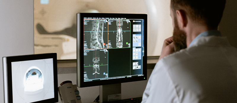
Although popular in its application, there is a major limitation of the projection radiography: the lack of depth resolution. Specifically, superimpositions of shadows from overlying and underlying tissues sometimes ''hide'' important details and limit contrast for medical diagnosis. To address this issue, a tomogram which is a 2-D image of a thin slice of the body is desirable. This is exactly what X-ray computed tomography (CT) does. The basic mechanism of CT is to use computer-processed combinations of multiple X-ray projections taken from different angles to produce tomographic images of a body, allowing the user to see inside the body without surgery. In contrast to projection radiography, the images in CT imaging are computed through mathematical manipulations of measurement data. In 1979, the Nobel Prize in Physiology or Medicine was awarded jointly to physicist Allan M CORMACK and electrical engineer Godfrey N HOUNSFIELD for the development of CT.

The math transforms behind CT

In a typical setting, a patient is rotated relative to the CT scanner, slightly around an axis running from head to foot between each X-ray projection to obtain a series of 2-D projections from different angles. Each horizontal line of the projection gives a 1-D projection of a 2-D axial cross section of the body at that angle. Thus, a collection of horizontal lines, one from each projection at the same height contains information about the axial cross section. This turns out to be exactly what 2-D Radon transform does. More precisely, the transform takes a function defined on the plane to a function defined on the space of lines in the plane whose value at a particular line is equal to the line integral of the function over the line. Using mathematical language, let be a function defined in , and the space of oriented lines in the plane be parameterised by the pairs 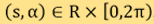where is the distance of the line from the origin and is the angle the normal vector of the line makes with X-axis. Then the Radon transform of , denoted by , is defined by

In CT, represents the attenuation coefficient of an axial cross section of the patient body, and what a CT scanner does is to sample its Radon transform at 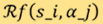for a discrete set of ray-paths represented by ’s at the angle . Radon transform was introduced in 1917 by mathematician Johann RADON, who also provided a formula for its inverse transform. It is this inverse transform that forms the basis for the widely used convolution back-projection (CBP) algorithms. The inversion formula reads as:

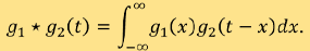
where is a 1-D function with Fourier transform , and “ ” denotes the convolution of two 1-D functions through the formula

It is worth mentioning that Radon transform can be generalised to higher dimensional Euclidean spaces and even Riemannian manifold. The properties of the transform are extensively studied in the mathematical field of integral geometry [5].

The math challenges of CT reconstruction

With the inversion formula (1), it seems easy to perform CT reconstruction. However, direct application of the formula usually yields poor quality images, in contrast to our expectations. The reason is that there are always noise in the measurement. What makes things worse is that the noise may be amplified by the inverse transform which is the convolution with the function . This is a typical feature of inverse problems; they are ill-posed. To be more precise, according to French mathematician Jacques HADAMARD's proposal, a problem is well-posed if the following three criteria are satisfied:

1. The problem must have a solution.
2. The solution must be unique.
3. The solution must be stable under small changes to the data.

On the other hand, a problem is called ill-posed if it violates one or more of the above criteria. At first, mathematicians thought problems that violated these criteria made no practical or physical sense, and that there was no need to attempt to find solutions to these problems. It has subsequently been shown, however, that mathematically ill-posed inverse problems are ubiquitous throughout science and engineering. Luckily, the ill-posed problems can be addressed by the powerful method of “regularisation" which seems to be a universal strategy. One of the most important examples is the Tikhonov regularisation which was first introduced by Russian mathematician and geophysicist Andrey Nikolayevich TIKHONOV. Regularisation is an extensively studied research field in inverse problems [3].

Back to our CT reconstruction problem, it falls into the ill-posed class by failing to satisfy the third criterion. A clever solution is provided by Ramachandranv and Lakshminarayan who replaced the convolution function with a new one referred to as the Ram-Lak filter. What the filter does is to mimic the behaviour of the function for its low frequency part while suppress its high frequency component. In this way, the part of the inverse transform which is not stable or sensitive to noise is regularised and the revised reconstruction formula can yield better images. Reconstruction methods of such type are called filtered back-projection. They are used in all commercial CT scanners in the past 40 years [6].

Better algorithms for better CT scanner?

Driven by the need to use less scanning time and to reduce the dose of X-ray radiation, CT systems are rapidly changing, and the once popular filter back-project algorithms are gradually giving way to new reconstruction methods. Take a 2-D case for example, we can first discretise the 2-D domain into pixels and approximate the attenuation function by the one which takes a constant value on each pixel. In this way, we can represent by a vector in . Each measurement gives a linear function of . With a total of M measurement, we get a system of linear equation with N unknowns, say,

where is the measurement matrix and corresponds to the measurement data. In typical situations, we have which corresponds to an image with resolution , and which corresponds to sampling 150 ray-paths at each of the 128 equally spaced angles. This is really a large system which cannot be directly inverted. In some more complicated scanning geometry where the image cannot be reconstructed slice by slice, the size of the system is even larger. The involved large computational cost seems to explain why the back-projection algorithms are still dominating in commercial CT systems. On the other hand, such large systems have drawn much research interest in the field of numerical linear algebra and many iterative techniques are developed to offer satisfactory solvers. One of them is Kaczmarz's method which was first discovered by the Polish mathematician Stefan KACZMARZ. Such methods relying on solving system of linear equations are called algebraic reconstruction techniques. It is worth mentioning that it is the algebraic reconstruction technique that was implemented in the first commercial CT scanner which is developed by Hounsfield. Compared to the back-projection based methods, iterative algorithms are favourable in reducing certain artefact and in dealing with noises. Moreover, their advantage is obvious in cases with partial or incomplete measurements where the inversion formula cannot be applied and in cases where one wants to reduce the X-ray doses without compromising the image qualify [4]. Reconstruction using partial measurement and achieving super-resolution without increase the X-ray doses give rises to new challenges since we have fewer equations than the number of unknowns. The reconstruction problem is even more ill-posed, but not without a solution. It is generally accepted that the number of freedoms in an image class, say human lungs for example, is much smaller than the number of total pixels in the image. Harnessing this problem-specific sparsity can essentially regularise the ill-posedness. In this respect, the theory of sparsity and compressed sensing [2] can provide the much-needed theoretical foundation. Reconstruction algorithms such as the iterative Sparse Asymptotic Minimum Variance can offer super-resolution imaging without requiring higher radiation dose and have attracted much research interest[1].

Concluding remark

CT is one of the most successful examples of inverse problems. Using mathematical modelling, most inverse problems in the real world can be viewed as a mathematical transform that maps physical parameters that are not directly observable to the measurements. Solving inverse problems is essentially finding the inverse transform. With the fundamental advances that have been made in the solution of inverse problems and the development of efficient numerical methods, we expect that these will eventually leads to breakthroughs in the reconstruction algorithms that allow us to see the inside world in a more friendly and healthier way without compromising the quality.

References

1. H. Abeida; Q. Zhang; J. Li and N. Merabtine, Iterative Sparse Asymptotic Minimum Variance Based Approaches for Array Processing, IEEE Transactions on Signal Processing. IEEE. 61 (4): 933-944, (2013).
2. D. L. Donoho, Compressed sensing, IEEE Transactions on Information Theory, vol. 52, no. 4, 1289-1306, (2006). doi: 10.1109/TIT.2006.871582.
3. H. W. Engl, M. Hanke and A. Neubauer, Regularization of Inverse Problems, Springer, Netherlands, (2000). ISBN 978-0-7923-4157-4.
4. C. L. Epstein, Introduction to the Mathematics of Medical Imaging, Societyfor Industrial and Applied Mathematics, 2nd Edition, (2007). ISBN: 978-0-89871-642-9.
5. S. Helgason, Integral Geometry and Radon Transforms, Springer, (2011). ISBN 9781441960542.
6. J. L. Prince and J. M. Links, Medical Imaging Signals and Systems, Pearson. 2nd edition, (2014). ISBN-13: 978-0132145183.

Author:
Prof ZHANG Hai, Associate Professor, Department of Mathematics, The Hong Kong University of Science and Technology

September 2021